Top Steps To Learn Naive Bayes Algorithm Free Download
What is the Naive Bayes Algorithm?
The naive Bayes poser, disregarding of the strong assumptions that it makes, is often exploited in practice, because of its simplicity and the small number classification of parameters required. The posture is in general exploited for classification — deciding, supported the values of the certify variables for a given instance, the class to which the exemplify is well-nig possible to go.
A Unworldly Bayes Classifier algorithmic rule supported Bayes theorem, which offers an perceptivity that IT is possible to adjust the probability of an issue A spick-and-span data introduces. It is a probabilistic algorithmic rule which means information technology calculates the probability of each tag for a given text, and then the output tag with the highest one. The algorithm is not a single nonpareil but a collection of different machine learning algorithms that use statistical Independence, which is easy to pen and run more efficiently than complex Bayes algorithms.
Functioning of Naive Bayes: Example
Classification
Suppose we undergo the dataset in which we have the prospect, the humidity and we necessitate to find whether we should play Oregon non on that day. The outlook could live a sunny overcast Beaver State rainy and the humidity is high or median. The wind is classified into two feeders which are weak winds and strong winds.
Dataset
| Twenty-four hour period | Outlook | Humidity | Wind | Bid |
| D1 | Sunny | Unpeasant-smelling | Perceptible | No |
| D2 | Bright | High gear | Strong | No |
| D3 | Overcast | Altitudinous | Weak | Yes |
| D4 | Rain down | High | Weak | Yes |
| D5 | Rain | Normal | Weak | Yes |
| D6 | Rain | Mean | Strong | No |
| D7 | Overcast | Normal | Strong | Yes |
| D8 | Sunny | High | Weak | No more |
| D9 | Sunny | Normal | Weak | Yes |
| D10 | Rain | Normal | Weak | Yes |
| D11 | Shiny | Normal | Strong | Yes |
| D12 | Overcast | High | Strong | Yes |
| D13 | Overcast | Natural | Weak | Yes |
| D14 | Rain | High | Rugged | No |
Frequency tables for apiece attribute of the data set are given as:

The succeeding are the Likeliness tables generated for all frequency table:
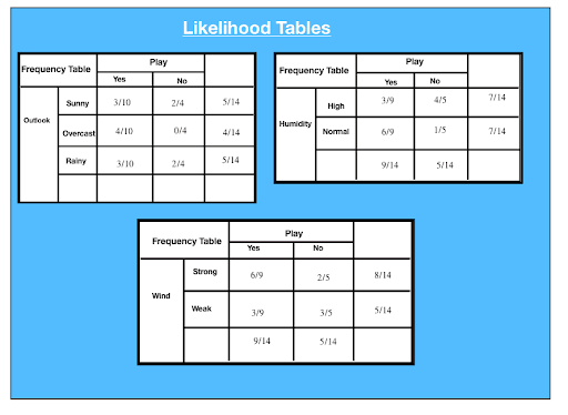
P(x|c) = P(Shiny|Yes) = 3/10 = 0.3
P(x) = P(Clear) = 5/14 = 0.36
P(c) = P(Yes) = 10/14 = 0.71
Attribute: Outlook: Clear
Likeliness of "Yes" given sunny is:
P(c|x) = P(Yes|Sunny) = P(Sunny|Yes) * P(Yes) | P(Shining)
= 0.3 x 0.71/ 0.36 = 0.591
Likelihood of "No" given sunny is:
P(c|x) = P(No|Sunny) = P(Sunny|No) * P(Zero) | P(Sunny)
= 0.4 x 0.36 / 0.36 = 0.40
Attribute: Humidity: Overlooking
Likelihood of "Yes" given high pressure humidity is:
P(c|x) = P(Yes|Humidity) = P(Humidity|Yes) * P(Yes) | P(Drunk)
= 0.33 x 0.6 / 0.36 = 0.42
Likeliness of "No" tending highschool humidness is:
P(c|x) = P(Nobelium|High) = P(High|No) * P(No) | P(Up).
= 0.8 x 0.36 / 0.5 = 0.58
Ascribe: Nose: Weak
Likelihood of "Yes" relinquished lame wind is:
P(c|x) = P(Yes|Humidity) = P(Humidity|Yes) * P(Yes) | P(Advanced)
= 0.67 x 0.64 / 0.57 = 0.75
Likelihood of "None" conferred pale wind is:
P(c|x) = P(No|Shrill) = P(High|Zero) * P(None) | P(High)
= 0.4 x 0.36/ 0.57 = 0.25
Reckon we deliver a day with the following values:
Outlook: Rain
Humidity: High
Roll: Weak
Play:?
Likelihood of 'No' connected that day.
P(Outlook= Rain down|No) * P(Humidity=High|No) * P(Wind = Weak|No) * P(No)

P(Yes)= 0.0199/ (0.0199 + 0.0166) = 0.55
P(Atomic number 102) = 0.0166 / (0.0199 + 0.0166)= 0.45
Thus, the model predicts that there is a 55% chance that there would be a game tomorrow.
Steps imply Naive Bayes Algorithm
EXAMPLE: PIMA DIABETIC TEST
The trouble comprises 768 observations of medical details of the patients' records describes instant measurement is confiscated from the patients such as they age, the number of times pregnant, blood workgroup. All the attributes are numeric and units vary from attribute to ascribe. Each commemorate has a class value that indicates whether the patients suffered on the set of diabetes within v years. The whole process can be brought down to fivesome steps:
Step 1: Handling Information
Information is loaded from the CSV File and spread into grooming and tested assets.
Footstep 2: Summarizing the Data
Summarise the properties in the preparation data localise to forecast the probabilities and make predictions.
Step 3: Making a Prediction
A particular prediction is successful using a summarise of the data set to make a single prediction.
Step 4: Making all the Predictions
Generate prediction given a test information set and a summarise data solidification.
Step 5: Evaluate Accuracy
Accuracy of the forecasting poser for the examine data situated as a per centum correct out of them all the predictions made.
Step 6: Tying all Together
Finally, we tie to all steps together and form our own model of Naive Thomas Bayes Classifier.
Encode
import csv
import random
meaning math
import numpy Eastern Samoa npdef load_csv(filename):
"""
:param filename: name of csv file
:return: data set arsenic a 2 dimensional list where each row in a list
"""
lines = csv.reader(open(filename, 'r'))
dataset = list(lines)
for i in range(len(dataset)):
dataset[i] = [plasterer's float(x) for x in dataset[I]]
comeback dataset
# data = load_csv('Pima-indians-diabetes.information.csv')
# print(data)def split_dataset(dataset, ratio):
"""
split dataset into training and testing
:param dataset: Two multidimensional list
:param ratio: Percent of information to go into the training set
:return: Training set and testing set
"""
size_of_training_set = int(len(dataset) * ratio)
train_set = []
test_set = tilt(dataset)
while len(train_set) < size_of_training_set:
index = random.randrange(len(test_set))
train_set.append(test_set.pop(index))
return [train_set, test_set]# training_set, testing_set = split_dataset(information, 0.67)
# photographic print(training_set)
# print(testing_set)def separate_by_label(dataset):
"""
:param dataset: two magnitude list of data values
:take back: dictionary where labels are keys and
values are the data points with that label
"""
separated = {}
for x in range(len(dataset)):
row = dataset[x]
if dustup[-1] not in separated:
separated[row[-1]] = []
separated[row[-1]].append(row)return separated
# separated = separate_by_label(data)
# print(separated)
# impress(separated[1])
# print(isolated[0])def calc_mean(last):
return tot(lst) / swim(len(last))
def calc_standard_deviation(in conclusion):
avg = calc_mean(last)
variance = sum([POW(x - avg, 2) for x in lst]) / float(len(lst) - 1)
return maths.sqrt(variance)# numbers racket = [1, 2, 3, 4, 5]
# print(calc_mean(numbers))
# print(calc_standard_deviation(numbers))def summarize_data(last):
"""
Calculate the think of and standard deviation for each dimension
:param lst: listing
:return: list with mean and orthodox deviation for each ascribe
"""summaries = [(calc_mean(attribute), calc_standard_deviation(attribute))
for property in energy(*lst)]
del summaries[-1]return summaries
# summarize_me = [[1, 20, 0], [2, 21, 1], [3, 22, 0]]
# print(summarize_data(summarize_me))def summarize_by_label(data):
"""
Method to resume the attributes for from each one label
:param data:
:return: dict label: [(atr mean, atr stdv), (atr mean, atr stdv)....]
"""
separated_data = separate_by_label(information)
summaries = {}
for label, instances in separated_data.items():
summaries[mark] = summarize_data(instances)
return summaries# fake_data = [[1, 20, 1], [2, 21, 0], [3, 22, 1], [4,22,0]]
# fake_summary = summarize_by_label(fake_data)def calc_probability(x, mean, standard_deviation):
"""
:param x: value
:param intend: average
:param standard_deviation: standardized deviation
:return: probability of that prise given a sane distribution
"""
# e ^ -(y - mingy)^2 / (2 * (standard deviation)^2)
exponent = math.exp(-(maths.pow(x - mean, 2) / (2 * math.pow(standard_deviation, 2))))
# ( 1 / sqrt(2π) ^ exponent
return (1 / (math.sqrt(2 * math.pi) * standard_deviation)) * exponent# x = 57
# mean = 50
# stand_dev = 5
# print(calc_probability(x, mean, stand_dev))def calc_label_probabilities(summaries, input_vector):
"""
the probability of a precondition information instance is deliberate by multiplying together
the attribute probabilities for to each one class. The result is a map of category values
to probabilities.
:param summaries:
:param input_vector:
:return: dict
"""
probabilities = {}
for label, label_summaries in summaries.items():
probabilities[mark] = 1
for i in grasp(len(label_summaries)):
mean, standard_dev = label_summaries[I]
x = input_vector[I]
probabilities[label] *= calc_probability(x, mean, standard_dev)return probabilities
# fake_input_vec = [1.1, 2.3]
# fake_probabilities = calc_label_probabilities(fake_summary, fake_input_vec)
# print(fake_probabilities)def anticipate(summaries, input_vector):
"""
Calculate the probability of a data instance belonging
to from each one label. We seek the largest probability and retrovert
the associated course.
:param summaries:
:param input_vector:
:render:
"""
probabilities = calc_label_probabilities(summaries, input_vector)
best_label, best_prob = None, -1
for label, chance in probabilities.items():
if best_label is None or probability > best_prob:
best_prob = probability
best_label = label
return best_label# summaries = {'A': [(1, 0.5)], 'B': [(20, 5.0)]}
# inputVector = 1.1
# print(predict(summaries, inputVector))def get_predictions(summaries, test_set):
"""
Make predictions for each information instance in our
test dataset
"""
predictions = []
for i in range(len(test_set)):
result = prefigure(summaries, test_set[i])
predictions.tack(result)riposte predictions
# summaries = {'A': [(1, 0.5)], 'B': [(20, 5.0)]}
# testSet = [1.1, 19.1]
# predictions = get_predictions(summaries, testSet)
# print(predictions)def get_accuracy(test_set, predictions):
"""
Compare predictions to class labels in the test dataset
and perplex our classification truth
"""
adjust = 0
for i in cast(len(test_set)):
if test_set[i][-1] == predictions[i]:
correct += 1return (correct / float(len(test_set))) * 100
# fake_testSet = [[1, 1, 1, 'a'], [2, 2, 2, 'a'], [3, 3, 3, 'b']]
# fake_predictions = ['a', 'a', 'a']
# fake_accuracy = get_accuracy(fake_testSet, fake_predictions)
# print(fake_accuracy)def independent(filename, split_ratio):
data = load_csv(filename)
training_set, testing_set = split_dataset(information, split_ratio)
print("Size of Training Set: ", len(training_set))
print("Size of it of Testing Dress: ", len(testing_set))# create model
summaries = summarize_by_label(training_set)# test mood
predictions = get_predictions(summaries, testing_set)
accuracy = get_accuracy(testing_set, predictions)
print('Accuracy: %'.format(accuracy))
primary('pima-indians-diabetes.information.csv', 0.70)
Pros of the Algorithm
- Naive Bayes Algorithm is a highly ascendable and fast algorithm.
- Binary star and Multiclass classification uses the Naive Bayes algorithm. GaussianNB, MultinomialNB, BernoulliNB are different kinds of algorithms.
- The algorithm depends on doing a cluster of counts.
- An excellent tasty for Text Classification problems. It's a popular choice for Spam electronic mail categorisation.
- Information technology can be easily trained on a small dataset.
Cons of the Algorithm
- According to the "Zero Contingent probability Problem.", if a presented feature and class have relative frequency 0, then the conditional chance estimate for that family comes out arsenic 0. This problem is cumbersome as it wipes out all the information in separate probabilities too. "Laplacian Fudge factor." is one of the try rectification techniques to fix this problem.
- Another con is that information technology makes a strong assumption of independence class features. It is nearly impossible to retrieve such data sets in veridical life.
Applications of Naive Bayes Algorithm
Uses of the Simple-minded Bayes algorithm in multiple real-life scenarios are:
- Textual matter classification: Used As a probabilistic scholarship method for text classification. The algorithm is the most successful algorithms when classifying text documents, i.e., whether a text document belongs to ace or more categories.
- Junk e-mail filtration: An example of textbook classification, is a popular mechanism to distinguish legitimate email from a spam e-mail. Many modern email services implement Bayesian spam filtering. Several waiter-side email filters, such atomic number 3 SpamBayes, SpamAssassin, DSPAM, ASSP, and Bogofilter, make use of this technique.
- Sentiment Analysis: It is wont to analyze the tone of tweets, comments, and reviews, i.e., whether they are positive, impersonal, or negative.
- Good word Organisation: The Naive Bayes algorithm, one with cooperative filtering, is used to make hybrid passport systems uses, which help oneself in predicting if a user would like a given resourcefulness or non
Conclusion
Hopefully, now you have understood what Naive Bayes is, and text classification makes use of goods and services of it. This simple method works considerably for sorting problems and, computationally speaking, information technology's also precise cheap. Whether the user is a Simple machine Learning expert or non, they have the tools to build their own Naive Bayes classifier.
Where answer you see this algorithmic rule at use? Net ball USA know! Commentary Below.
People are also reading:
- Python for Information Science
- Data Science Certification
- Information Science Degree
- Statistics for Data Science
- Information Science Tools
- Information Science Books
- What is Data Science?
- R for Data Science
DOWNLOAD HERE
Top Steps To Learn Naive Bayes Algorithm Free Download
Posted by: johnsonshood1961.blogspot.com
Post a Comment for "Top Steps To Learn Naive Bayes Algorithm Free Download"